Gravitational waves from dark domain walls

Abstract

This page gives an introduction to the production of Gravitational Waves (GWs) from the (a)symmetron dark energy model, and summarises and visualises the work performed in our paper on modelling and extrapolating the GW production. The code, 'AsGRD', that evolves the tensor perturbations, extends upon the code 'asevolution' that is introduced in the previous paper. The simulations that we show below are produced and presented in the companion paper and the corresponding webpage. In addition, we will introduce some illustrations and animations further visualising the simulations. The larger idea of this project is to explore for the first time in self-consistent simulations cosmological topological defects in the late-time universe as sources of gravitational waves.

Structure formation

The (a)symmetron dark energy model is a model of an additional scalar field in the matter sector, that has a non-minimal coupling to the trace of the stress-energy tensor of the rest of the matter sector. See this webpage for a more in-depth explanation. The coupling to the matter makes the field environmentally dependent, making it inactive in high-density regions and in the early universe. The post-inflationary universe is dense and nearly homogeneous. As matter dilutes due to cosmological expansion, the average density drops. Simultaneously, gravitational collapse increases the density contrasts and makes the matter field more inhomogeneous and eventually non-linear, creating the cosmic web and filaments. The matter density field \(\rho_m\) for this process, from cosmological redshift \(z=12\) to \(z=2.5\), is shown in the animation below.

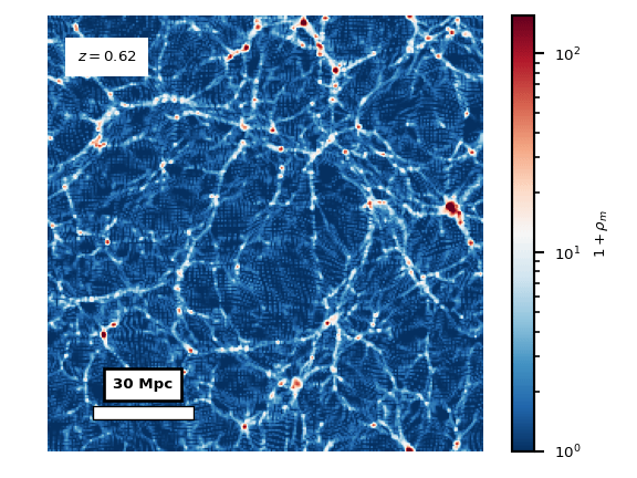
The animations above visualise the process of structure formation in the event of the standard cosmological scenario of a cosmological constant \(\Lambda\) and Cold Dark Matter (\(\Lambda\)CDM). In the event of the symmetron model, the repulsive nature of the void is enhanced, as can be seen in the animation below.

In comparison to the case of \(\Lambda\)CDM, we notice almost empty voids in the end of the animations. On the left-hand side, we have shown the field value of the symmetron field, normalised to its vacuum expectation value \(\chi\equiv \phi/v\). After the symmetry-breaking, we expect the field to take on the values \(\chi\rightarrow\pm 1\), depending only the local phase of its oscillations at the time of the symmetry breaking. The parameters for the above, small-box simulation are chosen as \(L_C,a_*,\beta_* = 750\) kpc, 1.25, 90 (See the paper for an in-depth explanation of the parameters). We emphasise that the choice of scale-factor at symmetry breaking \(a_*=1.25>1\) naively would mean that the phase transition should happen in the future. However, this mapping is done on the background, and due to the large density contrasts in the late-time structure formation, one will still get local symmetry breaking inside of the largest voids before this time.

Gravitational waves

In the below, we visualise the production of gravitational waves by showing animations in time of spatial slices of the simulations volume. On these slices, we show the self-contracted, time-differentiated tensor perturbations \(\dot{h}_{ij}\dot{h}^{ij}\), relating to the energy density of the GWs. We normalise it to the Hubble horizon \(H(z)\) so that it is a dimensionless quantity.

To create the sound, at first a white noise signal is generated, and then a band-pass filter is applied to match it to the power \(\dot{h}_{ij}\dot{h}^{ij}\) spectrum amplitudes. The filter is continuously adjusted as the video progresses, following the changes in the power spectrum. The frequency was shifted by 18 orders of magnitude, such that \(10^{-15}\) Hz becomes 1 kHz. This is a handy way to visualise the simulation spectra, but the correspondence to the videos should not be exact, because 1) videos are of slices of the simulation volume, whereas the spectra are of the entire box, and 2) the power spectra remove all non-Gaussian information originally contained within the fields' statistics.

\(\Lambda\)CDM

For the standard cosmological model, \(\Lambda\)CDM, we are seeing a mostly adiabatic evolution, but also a sourcing from the clustering cold dark matter. The amplitude for small scale modes is however very subleading with respect to the case of the other models.

One can also see faint ripples from fixed locations, throughout the simulation. These have been identified to be owing to the discretised mass distribution, and are caused by sudden displacements of particles when projected onto the lattice. The ripples' intensity was reduced significantly by going from a Nearest Grid Point (NGP) scheme to a higher order Cloud-In-Cell (CIC) scheme, and has been found to be unimportant with respect to the wave mode scales that we are interested in.

Model Z

\(\ (L_C, z_*, \bar \beta, \Delta \beta/\bar\beta)=(1\) Mpc/h\(\ , 2, 1, 0) \)

For a first demonstration of the production of gravitational waves from the scalar field, we show the case of a relatively early phase transition, at \(z_{SSB}=z_*=2\). In this event, we see a much more violent phase transition that is less confined by the environment and cosmic filaments. Instead, the resultant domain walls wander accross the simulation volume and eventually collapse, producing large ripples in both the scalar field and in the gravitational waves. The scale of these large domain collapses are comparatively larger, so that we would need a much larger box to resolve their statistics, but are instead resolving a single event here. Additionally, there is GW production from the vibrations of the walls that we are resolving the statistics of, and that we study in the other simulations below.

Model Ⅰ

\(\ (L_C, z_*, \bar \beta, \Delta \beta/\bar\beta)=(1\) Mpc/h\(\ , 0.1, 8, 0) \)

In this parameter choice, and the following ones, the symmetry breaking happens within the voids because of the density contrasts. Model Ⅰ is the fiducial choice for the large box simulations of the paper . The rest of the simulations vary on this by one parameter at the time.

Model Ⅱ

\(\ (L_C, z_*, \bar \beta, \Delta \beta/\bar\beta)=(0.75\) Mpc/h\(\ , 0.1, 8, 0) \)

In this case, we look for the effect of reducing the Compton wavelength \(L_C\) corresponding the to the Lagrangian mass parameter \(\mu\) and relating to the scale of correlation for the field when in vacuum. In this case, we expect a shift of the spectrum towards smaller scales. We are also seeing a different collapse of the scalar field due to different phases at the time of the symmetry breaking.

Model Ⅲ

\(\ (L_C, z_*, \bar \beta, \Delta \beta/\bar\beta)=(1\) Mpc/h\(\ , 0.1, 8, 10\%) \)

For the final animation that we display here, we show the effect of including an asymmetric potential \(\Delta\beta/\bar\beta=10\)%. The main effect seems to be more unstable domain walls, and therefore more collapses in the late-time universe, when the domains intersect more strongly.

Finally, for this same parameter choice, we demonstrate the behaviour of the tensor perturbation, contracted with the direction vector of the line of sight for an observer at equidistant shells moving from a distance \(D=370\) Mpc and source redshift \(z=0.08\) to an inner distance \(D=0\) Mpc and observer redshift \(z=0\). The contraction of the time-differentiated perturbation with the line of sight vector, is what should be integrated over the light path from the pulsars to the observer, to give the observable \(\Delta P/P\) that NANOGrav is measuring and doing statistics on (where \(P\) is the pulsar period).